Investment A [slide 42]-Grinold(Eqs. 17.20 to 17.23 [page 500])

[mikey10011]

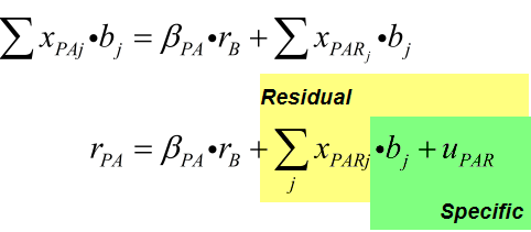
I am missing something with the substitutions so could you go through step-by-step equations 17.20 through 17.23 in Grinold (p. 500)? Also could you provide some insight or interpretation of the mathematical manipulations? For example where did u_PAR(t) in Eq. 17.23 come from?

Note that I bought Grinold Chapter 17 from GARP but the whole book is online with Google books (e.g., r_B(t) = benchmark return defined on p. 29). So feel free to refer to other pages outside of the chapter.

 

[David Harper CFA FRM]

Hi Mikey,

Good focus. IMO, Grinold Chapter 17 is pretty much about formula 17.23.

17.20 starts with a mutlifactor model (i.e., think CAPM but with additional factors). The active return (r_pa) is the sum of factor exposure (instead of market exposure in CAPM, replace exposure to benchmark) plus a residual (u_pa). So, the "leftover" u_pa in 17.2 is a residual.

Now consider these formulas that I copied below:

http://learn.bionicturtle.com/images/forum/grinold_17.23.png

Please note, in the first line above, the generic factor exposure in 17.20 (x_pa) is broken into two pieces: the active systemic return which is exposure to the benchmark (B_pa*r_pa) and the common factor exposure (x_par). The x_par refers to factor exposures which are NOT the benchmark.

The right-hand side of the top formula above is substituted into 17.20: the generic factor exposures are parsed into systemic/benchmark plus common/non-benchmark. That's really all that happens from 17.2 to 17.23. When this is substituted into 17.20, there is still a "left over" piece: the "left-over" just now becomes the SPECIFIC in 17.23. In both cases, the u_pa and the u_par are the returns that don't correlate with any factor specified by the model.

At the end (17.23, or my second line above) we really just have a multi-factor model. I do think it helps to recognize the intuition of the middle term (x_par): these are factors that correlate to portfolio returns but they are non-benchmark factors. Whereas beta_pa is correlation to benchmark.

In summary,

The RESIDUAL (u_pa) in 17.2 becomes the SPECIFIC (u_par) in 17.23; both are uncorrelated to benchmark/common factors
The generic factor (x_pa) in 17.2 breaks into SYSTEMIC/benchmark (beta_pa) and COMMON/non-benchmark (x_par)
The RESIDUAL in 17.23 includes both the common factors (x_par) and the SPECIFIC return because in 17.20 the active beta is trapped inside the x_pa, but it is released by parsing out the common factors. So, the RESIDUAL in 17.23 is still the part not explained by exposure to the benchmark but now it is also not explained by common factors. It starts (17.2) being the part not explained by generic factors; it finishes (17.23) being the part not explained by either correlation to benchmark or correlation to common factors.

Sometimes i think the math makes this more complicated than it needs to be. We start (17.2) with returns that are (i) correlated to generic factors or (ii) un-correlated. Then by parsing the generic factors into benchmark and common, we end up with returns that are (i) correlated to the benchmark, (ii) correlated to non-benchmark common factors or (iii) neither of the above (residual).

David