P1 Focus Review, 2nd of 8 (Quantitative Econometrics): Videos, Practice Questions and Learning Spreadsheets
The Quantitative Topic (T2) is large so it will be divided over two focus reviews. This Review covers Stock & Watson's Econometrics, which I reduce to the following:
You absolutely need to know the basic properties of variance and covariance. Please make sure you are comfortable with:
Exam-wise the most likely applications here are: compute a mean (expected value) or compute a variance. An extremely popular question asks to find the variance of a two-asset portfolio, which employs the variance property above. BTW, can you employ it if one of the positions is a short position? (see this question which is formally P2 but could fall under P1 also: http://forum.bionicturtle.com/threads/professor-jorion-chapter-7.6139/)
Also, please get very comfortable with:
Here in introductory econometrics, we care mostly about the so-called sampling distributions:
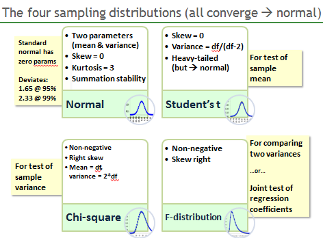
In the exam, you are overwhelming likely to encounter two distributions:
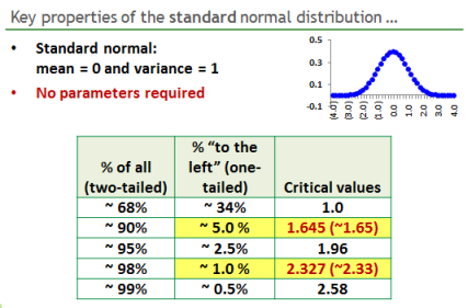
These standard normal deviates get us the most common FRM P1 metric: normal (parametric) value at risk (VaR) which is simply volatility scaled by a deviate (which is a function of desired confidence):
Inference
The essential formula here is the standardization of an observed sample mean with: t = (observed sample mean - hypothesized mean)/standard error. The popular test is whether a coefficient is significant; that is, null hypothesis, H(0): population mean = zero.
A common application (e.g., regression) is then to divide the observed sample mean by the standard error, which really just produces a standard standard deviation. If this test statistic is really high (e.g., double digits), we can reject the null because we are far into the tail. If this statistic is low (e.g., below 2.0), our sample mean is not very far away from oour hypothesized mean, and we probably can't reject the null.
Other highly testable concepts here are:
Regression
Historically, the FRM has over-assigned regression, testing the superficial application and not testing the layer of theory. So, the essentials include:
- The Part 1 (P1) 2nd (of 8) Focus Review video (Econometrics) is available here
- We've streamlined (and updated) the associated Practice Questions into a single set, here at P1.T2. Stock, Chapters 2-7 (55 pages!)
- We will be restoring, also, a consolidated set of Gujarati Practice Questions. I do strongly agree with LL that our historical set of Gujarati questions are highly relevant (see http://forum.bionicturtle.com/threads/gujarati.6132/)
- I am still updating the Learning Spreadsheets (in the meantime, 2011 XLS still apply)
The Quantitative Topic (T2) is large so it will be divided over two focus reviews. This Review covers Stock & Watson's Econometrics, which I reduce to the following:
- Random variables
- Distributions
- Inference
- Regression
You absolutely need to know the basic properties of variance and covariance. Please make sure you are comfortable with:
- variance (aX + bY) = a^2*variance(X) + b^2*variance(Y) + 2*A*B*covariance(X,Y). And really handy is:
- covariance(X,Y) = E[X*Y] - E[X]*E[Y]. Note, for example we can use this (i) to infer expected loss (EL) when PD*LGD are correlated and (ii) to find that Variance(X) = E[X^2] - (E[X])^2
Exam-wise the most likely applications here are: compute a mean (expected value) or compute a variance. An extremely popular question asks to find the variance of a two-asset portfolio, which employs the variance property above. BTW, can you employ it if one of the positions is a short position? (see this question which is formally P2 but could fall under P1 also: http://forum.bionicturtle.com/threads/professor-jorion-chapter-7.6139/)
Also, please get very comfortable with:
- Marginal (i.e. unconditional) probability, versus
- Conditional probability, versus
- Joint probability
Here in introductory econometrics, we care mostly about the so-called sampling distributions:
In the exam, you are overwhelming likely to encounter two distributions:
- Normal, and
- Student's t: because this is for a test of the sample mean when we don't know the population variance
These standard normal deviates get us the most common FRM P1 metric: normal (parametric) value at risk (VaR) which is simply volatility scaled by a deviate (which is a function of desired confidence):
- 99% VaR = 2.33*volatility, because if returns are normal, only 1% of the returns should fall into one-side tail which is 2.33 standard deviations away from the mean.
Inference
The essential formula here is the standardization of an observed sample mean with: t = (observed sample mean - hypothesized mean)/standard error. The popular test is whether a coefficient is significant; that is, null hypothesis, H(0): population mean = zero.
A common application (e.g., regression) is then to divide the observed sample mean by the standard error, which really just produces a standard standard deviation. If this test statistic is really high (e.g., double digits), we can reject the null because we are far into the tail. If this statistic is low (e.g., below 2.0), our sample mean is not very far away from oour hypothesized mean, and we probably can't reject the null.
Other highly testable concepts here are:
- Type I and Type II error, and
- Interpretation of p-value (my tip is to think "I can reject the null with 1-p confidence or lower confidence [but not any higher confidence]")
Regression
Historically, the FRM has over-assigned regression, testing the superficial application and not testing the layer of theory. So, the essentials include:
- Make sure you can interpret a linear regression; e.g., can you say what B2 means in the multivariate Y(i) = B(0) + B(1)*X(1i) + B(2)*X(2i) + ... B(k)*X(ki)
- Make sure you can solve for the dependent (application of linear regression output)
- I would understand homoskedasticity (is it a violation of an OLS assumption? If so, specifically how?)
- You must know that R^2 = ESS/TSS = 1 - SSR/TSS (don't forget that in a univariate regression, R^2 is the square of the correlation coefficient)
- In the video, I finished with a regression example. You do want to get comfortable with: looking at a regression output and being able to figure whether the coefficients are significant.