Learning objectives: Use sample data to estimate quantiles, including the median. Estimate the mean of two variables and apply the CLT. Estimate the covariance and correlation between two random variables. Explain how coskewness and cokurtosis are related to skewness and kurtosis.
Questions:
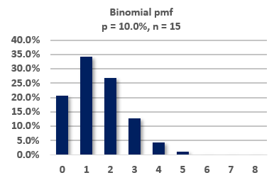
20.13.1. Below is the probability mass function (pmf) of a binomial random variable where the probability of success over 15 trials is 10.0%; i.e., p = 0.10 and n = 15.

What is the interquartile range (IQR) of this probability distribution?
a. Zero
b. 1.0
c. 2.5
d. 4.0
20.13.2. Consider two different mutual funds and their respective monthly standard deviations over the last 48 months (sample size, n = 48):
Recall that the variance between differences is given by σ^2(X - Y) = σ^2(X) + σ^2(Y) - 2*COV(X,Y). Further, the central limit theorem (CLT) says that, under conditions, the standard error of the sample mean is given by SQRT(σ^2/n) or σ/SQRT(n). We only need these two concepts, and to keep in mind that we are now treating each fund's sample mean as a random variable, to answer the question: which of the following is nearest to the standard error (aka, standard deviation) of the difference between these two funds' sample means?
a. 0.035% or 0.00035
b. 0.197% or 0.00197
c. 0.700% or 0.00700
d. 0.842% or 0.00842
20.13.3. Below is a scatterplot of monthly returns, Fund A versus Fund B, over twenty months (n = 20).

Skewness is a trivial (special) case of coskewness; e.g., S(AAA) and S(BBB) are the trivial instances of coskewness. Similarly, Kurtosis is the trivial case of coskewness; e.g., K(AAAA) and K(BBBB) are the trivial instances of cokurtosis. In regard to this scatterplot (this two-variable application), how many nontrivial coskewness measures apply; are they positive or negative; and how many nontrivial cokurtosis measures exist?
a. There are two nontrivial coskewness measures and they are negative (aka, negative coskewness); there are three nontrivial cokurtosis measures
b. There are three nontrivial coskewness measures and they are negative (aka, negative coskewness); there are four nontrivial cokurtosis measures
c. There are two nontrivial coskewness measures and they are positive (aka, positive coskewness); there are five nontrivial cokurtosis measures
d. There are three nontrivial coskewness measures and they are positive (aka, positive coskewness); there are six nontrivial cokurtosis measures
Answers here:
Questions:
20.13.1. Below is the probability mass function (pmf) of a binomial random variable where the probability of success over 15 trials is 10.0%; i.e., p = 0.10 and n = 15.

What is the interquartile range (IQR) of this probability distribution?
a. Zero
b. 1.0
c. 2.5
d. 4.0
20.13.2. Consider two different mutual funds and their respective monthly standard deviations over the last 48 months (sample size, n = 48):
- Fund A has a monthly volatility of 3.0%, and
- Fund B has a monthly volatility of 5.0%.
Recall that the variance between differences is given by σ^2(X - Y) = σ^2(X) + σ^2(Y) - 2*COV(X,Y). Further, the central limit theorem (CLT) says that, under conditions, the standard error of the sample mean is given by SQRT(σ^2/n) or σ/SQRT(n). We only need these two concepts, and to keep in mind that we are now treating each fund's sample mean as a random variable, to answer the question: which of the following is nearest to the standard error (aka, standard deviation) of the difference between these two funds' sample means?
a. 0.035% or 0.00035
b. 0.197% or 0.00197
c. 0.700% or 0.00700
d. 0.842% or 0.00842
20.13.3. Below is a scatterplot of monthly returns, Fund A versus Fund B, over twenty months (n = 20).

Skewness is a trivial (special) case of coskewness; e.g., S(AAA) and S(BBB) are the trivial instances of coskewness. Similarly, Kurtosis is the trivial case of coskewness; e.g., K(AAAA) and K(BBBB) are the trivial instances of cokurtosis. In regard to this scatterplot (this two-variable application), how many nontrivial coskewness measures apply; are they positive or negative; and how many nontrivial cokurtosis measures exist?
a. There are two nontrivial coskewness measures and they are negative (aka, negative coskewness); there are three nontrivial cokurtosis measures
b. There are three nontrivial coskewness measures and they are negative (aka, negative coskewness); there are four nontrivial cokurtosis measures
c. There are two nontrivial coskewness measures and they are positive (aka, positive coskewness); there are five nontrivial cokurtosis measures
d. There are three nontrivial coskewness measures and they are positive (aka, positive coskewness); there are six nontrivial cokurtosis measures
Answers here:
Last edited by a moderator:
