Learning objectives: Describe the requirements for a series to be covariance stationary. Define the autocovariance function and the autocorrelation function. Define white noise; describe independent white noise and normal (Gaussian) white noise.
Question:
20.21.1. Pamela has been tasked to simulate a set of economic variables over time. She considers the following eight time-series processes as candidates for her model:
Which is (are) covariance stationary?
a. Only one of these (i.e., 1 of 8) is covariance stationary
b. A minority of these (i.e., 2 or 3) are covariance stationary
c. A majority of these (i.e., 6 of 8) are covariance stationary
d. All of these (i.e., 8 of 8) processes are covariance stationary
20.21.2. Shown below is the autocorrelation function (ACF) for a time series object that contains the total quarterly beer production in Australia (in megalitres) from 1956:Q1 to 2010:Q2 (source: https://cran.r-project.org/web/packages/fpp2/index.html).
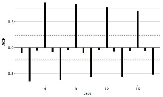
About this ACF and its implications, each of the following statements is true EXCEPT which statement is false?
a. ρ(1) and ρ(3) are insignificant
b. This time series is a white noise process
c. This ACF is compatible with a seasonal time series
d. If this time series exhibits stochastic seasonality, it might be possible to fit a seasonal ARMA model
20.21.3. Barbara was delighted to learn that she can easily simulate white noise in R with a single command. She learned that she can use arima.sim(model = list(order = c(0,0,0)), n = 100) to generate white noise with an ARIMA(0,0,0) model over a length of 100 days. She wants the shocks to have a Poisson distribution so she uses the command arima.sim(model = list(order = c(0,0,0)), n = 100, rand.gen = function(n, ...) rpois(n, lambda = 10)) which assumes a Poisson distribution. Below is a plot of the white noise (top panel) and its associated autocorrelation function (ACF, bottom panel).

Is Barbara's time series model a genuine white noise (WN) process?
a. Yes, Barbara's simulation is white noise: although the series has a non-zero mean it can easily be defined in terms of a mean-zero error
b: Yes, Barbara's simulation is white noise: this series has heteroskedasticity and positive auto-covariance which are both valid features of white noise
c. No, Barbara's simulation is not white noise because white noise must be independent and the lower panel proves this series is not white noise
d No, Barbara's simulation is not white noise because white noise requires that she assume the distribution function is normal but the shocks in her series are non-normal
Answers here:
Question:
20.21.1. Pamela has been tasked to simulate a set of economic variables over time. She considers the following eight time-series processes as candidates for her model:
I. White noise, ε(t) ∼ WN(0, σ^2)
II. Random walk, X(t) = X(t-1) + ε(t)
III. First difference of random walk, X(t) - X(t-1)
IV. First difference of random walk with trend
V. Stock prices under lognormal property where S(t) = S(0)*exp(μ + σ*Z)
VI. The log returns (aka, geometric returns) under lognormal property where S(t) = S(0)*exp(μ + σ*Z)
VII. First-order autoregressive process, AR(1), with AR parameter |ϕ| < 1
VIII. First-order moving average process, MA(1), with non-zero mean, μ <> 0
Which is (are) covariance stationary?
a. Only one of these (i.e., 1 of 8) is covariance stationary
b. A minority of these (i.e., 2 or 3) are covariance stationary
c. A majority of these (i.e., 6 of 8) are covariance stationary
d. All of these (i.e., 8 of 8) processes are covariance stationary
20.21.2. Shown below is the autocorrelation function (ACF) for a time series object that contains the total quarterly beer production in Australia (in megalitres) from 1956:Q1 to 2010:Q2 (source: https://cran.r-project.org/web/packages/fpp2/index.html).
About this ACF and its implications, each of the following statements is true EXCEPT which statement is false?
a. ρ(1) and ρ(3) are insignificant
b. This time series is a white noise process
c. This ACF is compatible with a seasonal time series
d. If this time series exhibits stochastic seasonality, it might be possible to fit a seasonal ARMA model
20.21.3. Barbara was delighted to learn that she can easily simulate white noise in R with a single command. She learned that she can use arima.sim(model = list(order = c(0,0,0)), n = 100) to generate white noise with an ARIMA(0,0,0) model over a length of 100 days. She wants the shocks to have a Poisson distribution so she uses the command arima.sim(model = list(order = c(0,0,0)), n = 100, rand.gen = function(n, ...) rpois(n, lambda = 10)) which assumes a Poisson distribution. Below is a plot of the white noise (top panel) and its associated autocorrelation function (ACF, bottom panel).
Is Barbara's time series model a genuine white noise (WN) process?
a. Yes, Barbara's simulation is white noise: although the series has a non-zero mean it can easily be defined in terms of a mean-zero error
b: Yes, Barbara's simulation is white noise: this series has heteroskedasticity and positive auto-covariance which are both valid features of white noise
c. No, Barbara's simulation is not white noise because white noise must be independent and the lower panel proves this series is not white noise
d No, Barbara's simulation is not white noise because white noise requires that she assume the distribution function is normal but the shocks in her series are non-normal
Answers here:
Last edited by a moderator: