Learning objectives: Describe the basic steps to conduct a Monte Carlo simulation. Describe ways to reduce Monte Carlo sampling error.
Questions:
21.5.1. Mary wants to approximate the expected value of an option. She conducts a Monte Carlo simulation and based on her initial sample size, n = 100, she estimates the fair value of the option is USD $72.00. The value is determined by taking the mean of the sample. She observes that the sample standard deviation is USD $29.00. She wants to obtain a 95.0% confidence interval (CI width in total) that is less than 5.0% of the option's fair value. If she makes an (unrealistic) assumption that the sample standard deviation will remain constant at $29.00 as she increases the sample size, what is nearest to her minimum desired sample size?
a. 50
b. 1,000
c. 20,000
d. 400,000
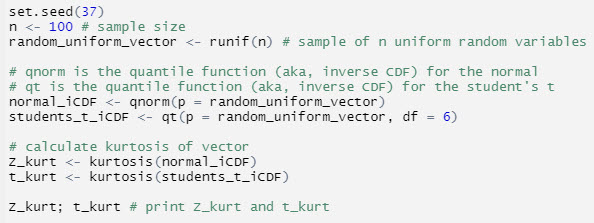
21.5.2. The following code snippet generates a vector of 100 random values from the uniform distribution--per a typical pseudo-random number generator--that serves as a vector of random probabilities from zero to 1.0; the function runif(n) generates a vector of n random numbers. From this vector of random probabilities are retrieved a vector of corresponding quantiles (aka, per the inverse cumulative distribution function or inverse CDF) according to two distributions: the normal and the student's t with six degrees of freedom, df = 6. The final two lines simply calculate the excess kurtosis of each sample: Z_kurt is the excess kurtosis of the sample of random normal variables, and t_kurt is the excess kurtosis of the sample of random student's t variables.

If we re-run this simulation (program) several times and observe the values, which of the following is most likely to be TRUE about the outputs Z_kurt and t_kurt?
a. Each run will produce different values of Z_kurt and t_kurt
b. Each run will produce exactly the following: Z_kurt = 0 and t_kurt = 3.0
c. The program will crash because set.seed(37) contradicts the random number generator
d. Each run will produce identical values of Z_kurt and t_kurt but it will be the case that Z_kurt <> 0 and t_kurt <> 3.0
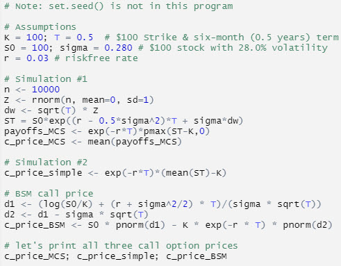
21.5.3. Nora wants to value a six-month at-the-money call option. Her program has five small sections and is displayed below. The first section ("Assumptions") assigns values to the inputs: S(0) = $100.00, K = $100,00, riskfree rate = 3.0%, volatility (sigma) = 28.0% and term to maturity = six months (0.5 years). The first simulation ("Simulation #1") generates the call prices (i.e., c_price_MCS) according to a Monte Carlo simulation. The second simulation ("Simulation #2") performs a very simple simulation to generate the call option price (i.e., c_price_simple). The next section computes the call option price (i.e., c_price_BSM) according to the Black-Scholes-Merton (BSM) option-pricing model. The final section simply prints the three different call prices that were obtained earlier: c_price_MCS, and c_price_simple, c_price_BSM.

About Nora's program and its approach to estimating the price of the six-month call option, each of the following statements is true EXCEPT which is false?
a. The first Monte Carlo simulation (#1), c_price_MCS, is correctly specified
b. The second simulation (#2), c_price_simple, is the best approach because it discounts the difference between the future mean stock price and the strike price
c. The analytical Black-Scholes, c_price_BSM, function is correctly specified
d. If we re-run the program several times, the BSM price (i.e., c_price_BSM) will repeat each time, but the simulated values (i.e., c_price_MCS) will differ on each run
Answers here:
Questions:
21.5.1. Mary wants to approximate the expected value of an option. She conducts a Monte Carlo simulation and based on her initial sample size, n = 100, she estimates the fair value of the option is USD $72.00. The value is determined by taking the mean of the sample. She observes that the sample standard deviation is USD $29.00. She wants to obtain a 95.0% confidence interval (CI width in total) that is less than 5.0% of the option's fair value. If she makes an (unrealistic) assumption that the sample standard deviation will remain constant at $29.00 as she increases the sample size, what is nearest to her minimum desired sample size?
a. 50
b. 1,000
c. 20,000
d. 400,000
21.5.2. The following code snippet generates a vector of 100 random values from the uniform distribution--per a typical pseudo-random number generator--that serves as a vector of random probabilities from zero to 1.0; the function runif(n) generates a vector of n random numbers. From this vector of random probabilities are retrieved a vector of corresponding quantiles (aka, per the inverse cumulative distribution function or inverse CDF) according to two distributions: the normal and the student's t with six degrees of freedom, df = 6. The final two lines simply calculate the excess kurtosis of each sample: Z_kurt is the excess kurtosis of the sample of random normal variables, and t_kurt is the excess kurtosis of the sample of random student's t variables.

If we re-run this simulation (program) several times and observe the values, which of the following is most likely to be TRUE about the outputs Z_kurt and t_kurt?
a. Each run will produce different values of Z_kurt and t_kurt
b. Each run will produce exactly the following: Z_kurt = 0 and t_kurt = 3.0
c. The program will crash because set.seed(37) contradicts the random number generator
d. Each run will produce identical values of Z_kurt and t_kurt but it will be the case that Z_kurt <> 0 and t_kurt <> 3.0
21.5.3. Nora wants to value a six-month at-the-money call option. Her program has five small sections and is displayed below. The first section ("Assumptions") assigns values to the inputs: S(0) = $100.00, K = $100,00, riskfree rate = 3.0%, volatility (sigma) = 28.0% and term to maturity = six months (0.5 years). The first simulation ("Simulation #1") generates the call prices (i.e., c_price_MCS) according to a Monte Carlo simulation. The second simulation ("Simulation #2") performs a very simple simulation to generate the call option price (i.e., c_price_simple). The next section computes the call option price (i.e., c_price_BSM) according to the Black-Scholes-Merton (BSM) option-pricing model. The final section simply prints the three different call prices that were obtained earlier: c_price_MCS, and c_price_simple, c_price_BSM.

About Nora's program and its approach to estimating the price of the six-month call option, each of the following statements is true EXCEPT which is false?
a. The first Monte Carlo simulation (#1), c_price_MCS, is correctly specified
b. The second simulation (#2), c_price_simple, is the best approach because it discounts the difference between the future mean stock price and the strike price
c. The analytical Black-Scholes, c_price_BSM, function is correctly specified
d. If we re-run the program several times, the BSM price (i.e., c_price_BSM) will repeat each time, but the simulated values (i.e., c_price_MCS) will differ on each run
Answers here:
Last edited by a moderator:
