Learning objectives: Explain how the principles of arbitrage pricing of derivatives on fixed-income securities can be extended over multiple periods. Define option-adjusted spread (OAS) and apply it to security pricing. Describe the rationale behind the use of recombining trees in option pricing. Calculate the value of a constant maturity Treasury swap, given an interest rate tree and the risk-neutral probabilities. Evaluate the advantages and disadvantages of reducing the size of the time steps on the pricing of derivatives on fixed-income securities. Evaluate the appropriateness of the Black-Scholes-Merton model when valuing derivatives on fixed-income securities.
Questions:
23.2.1. Below is a multi-period price tree for a zero-coupon bond with 1.5 years to maturity. It is similar to Tuckman's (4th edition); in fact, the only difference (among assumptions) is that the spot rate term structure below has been shifted up in parallel by 100 basis points. Specifically, the spot rate term structure below is given by {3.0% @ 0.5 years, 3.15% at one year, and 3.25% at 1.5 years}.
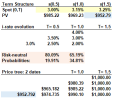
In regard to this multi-period tree, each of the following statements is true EXCEPT which is false?
a. The bond's current market price of $952.79 assumes real-world probabilities applied to its expected discounted value (EDV)
b. If there is an increase in the 1.5-year spot rate, S(1.5), from 3.25% to 3.50%, this will impact (at least some of) the risk-neutral probabilities
c. The drifts (aka, expected changes) in the six-month rate are +30.1 basis points (from date 0 to 1) and 15.2 basis points (from dates 1 to 2)
d. To extend the tree to any number of further dates (e.g., 2 years with a date 4 column, 2.5 years with a date 5 column) requires assumptions about the future possible values of the short‐term rate and the calculation of risk‐neutral probabilities that recover a given set of bond prices
23.2.2. Below is the price tree for a stylized constant-maturity Treasury (CMT) swap struck at 2.0% with a notional of $1.0 million. The risk-neutral probabilities are displayed, specifically: 80.09% (d = 19.91%) from date 0 to date 1; and 65.20% (d = 34.80%) from date 1 to date 2. Using these risk-neutral probabilities returns an expected discounted value (EDV) of $3,702.11 for the value of the CMT swap. Please notice this exactly matches Tuckman's Figure 7.8 in his 4th edition value. This is the so-called model value.
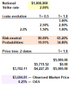
Assume the observed market price of this CMT swap is $3,694.81 (as highlighted in purple), which is $7.30 less than the market price. This implies an option-adjusted spread (OAS) of 25 basis points. Which of the following is the best interpretation of this OAS?
a. The model returns the market price if we adjust the risk-neutral probabilities to 55.09% and 44.91%
b. The model returns the market price if we assume adjusted cash flows; e.g., $3,750 instead of $5,000 on (state 2, date 2)
c. The model returns the market price if we use discount rates of 2.25% (date 0, state 0), 1.75% (date 1, state 0), and 2.75% (date 1, state 1)
d. We cannot interpret the OAS here because this is a CMT swap, and the OAS requires an embedded option; e.g., a bond with an embedded call option
23.2.3. Below are price trees for two $1,000 face value zero-coupon bonds with maturities, respectively, of one year and 1.5 years.
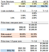
According to this binomial tree, what is (are) the implied one-year forward rate(s), F(0.5, 1.0)?
a. A single one-year forward rate: F(0.5, 1.0) = 3.075%
b. One of two possible forward rates: F(0.5, 1.0) will be either 2.575% or 3.575%
c. One of three possible forward rates: F(0.5, 1.0) will be either 1.75%, 2.50%, or 3.25%
d. It is impossible to infer F(0.5, 1.0) as there are virtually infinite possible forward rates
Answers:
Questions:
23.2.1. Below is a multi-period price tree for a zero-coupon bond with 1.5 years to maturity. It is similar to Tuckman's (4th edition); in fact, the only difference (among assumptions) is that the spot rate term structure below has been shifted up in parallel by 100 basis points. Specifically, the spot rate term structure below is given by {3.0% @ 0.5 years, 3.15% at one year, and 3.25% at 1.5 years}.

In regard to this multi-period tree, each of the following statements is true EXCEPT which is false?
a. The bond's current market price of $952.79 assumes real-world probabilities applied to its expected discounted value (EDV)
b. If there is an increase in the 1.5-year spot rate, S(1.5), from 3.25% to 3.50%, this will impact (at least some of) the risk-neutral probabilities
c. The drifts (aka, expected changes) in the six-month rate are +30.1 basis points (from date 0 to 1) and 15.2 basis points (from dates 1 to 2)
d. To extend the tree to any number of further dates (e.g., 2 years with a date 4 column, 2.5 years with a date 5 column) requires assumptions about the future possible values of the short‐term rate and the calculation of risk‐neutral probabilities that recover a given set of bond prices
23.2.2. Below is the price tree for a stylized constant-maturity Treasury (CMT) swap struck at 2.0% with a notional of $1.0 million. The risk-neutral probabilities are displayed, specifically: 80.09% (d = 19.91%) from date 0 to date 1; and 65.20% (d = 34.80%) from date 1 to date 2. Using these risk-neutral probabilities returns an expected discounted value (EDV) of $3,702.11 for the value of the CMT swap. Please notice this exactly matches Tuckman's Figure 7.8 in his 4th edition value. This is the so-called model value.

Assume the observed market price of this CMT swap is $3,694.81 (as highlighted in purple), which is $7.30 less than the market price. This implies an option-adjusted spread (OAS) of 25 basis points. Which of the following is the best interpretation of this OAS?
a. The model returns the market price if we adjust the risk-neutral probabilities to 55.09% and 44.91%
b. The model returns the market price if we assume adjusted cash flows; e.g., $3,750 instead of $5,000 on (state 2, date 2)
c. The model returns the market price if we use discount rates of 2.25% (date 0, state 0), 1.75% (date 1, state 0), and 2.75% (date 1, state 1)
d. We cannot interpret the OAS here because this is a CMT swap, and the OAS requires an embedded option; e.g., a bond with an embedded call option
23.2.3. Below are price trees for two $1,000 face value zero-coupon bonds with maturities, respectively, of one year and 1.5 years.

According to this binomial tree, what is (are) the implied one-year forward rate(s), F(0.5, 1.0)?
a. A single one-year forward rate: F(0.5, 1.0) = 3.075%
b. One of two possible forward rates: F(0.5, 1.0) will be either 2.575% or 3.575%
c. One of three possible forward rates: F(0.5, 1.0) will be either 1.75%, 2.50%, or 3.25%
d. It is impossible to infer F(0.5, 1.0) as there are virtually infinite possible forward rates
Answers:
Last edited:
