David Harper CFA FRM

David Harper CFA FRM
Subscriber
In our latest Week in Financial Education (WIFE), Richie's new video helpfully reviews a series of duration questions, including modified, Macaulay, money duration and price value of basis point (PVBP; aka, PV01). Compared to the FRM, the CFA's approach to duration differs only slightly. The formulas are essentially similar. The CFA's modified duration is analytical (e.g., solved functionally) while its approximate modified duration is called effective duration in the FRM (i.e., approximated or simulated by shocking an interest rate factor). The CFA's approximate modified duration shocks the yield (reprices the bond) while its effective duration instead re-prices a term structure (aka, benchmark curve). However--as far as I can tell--both are parallel shifts (geeky note: a parallel shift implies single-factor but single-factor models can be non-parallel). For myself, I do not view the CFA's distinction between approximate modified duration and effective duration (which are both effective duration in the FRM; the FRM starts from a fairly generalized interest rate factor/vector) as highly consequential. They are both durations approximated via a parallel shift. New learners should be able to see that most of these vocabularies refer to different approaches around the same single concept, but measured in different ways (as a percentage, a time/maturity, or a dollar implication). You've got to do the practice just like Richie shows us. Finally, the FRM's dollar duration is called money duration in the CFA. It gets less attention (mathematically this is the tangent line's negated slope, less prone to interpretation, but it's just a rescaled PVBP * 10,000 because there are 10,000 basis points in 100.0%) but money duration/PVBP are arguably the most useful because we use them to hedge.

I hope you like the new practice question sets. I am happy with the code snippet that illustrates an antithetic variate: you don't need code background to follow this super simple example. Question 21.6.2. also employs a code snippet, but notice how you don't really need it to answer the question! I am trying to give us practice that is useful. Simulation is not a passive reading exercise, it is done in code. You can spend an entire day reading about bootstrapping and you may never learn it. Bootstrapping is truly a doing thing. I actually put much effort into writing brief snippets (with comments) in the hopes they serve you with realistic examples. Have a good study week!

New YouTube
New Practice Question Sets
In the forum
Curated Links
 
Last edited by a moderator:

David Harper CFA FRM

David Harper CFA FRM
Subscriber
Note: An addition to our CAPM Learning Spreadsheet

We received a question on YouTube that is helpful in understanding the relationship (and difference) between the Capital Market Line (CML) and the Security Market Line (SML). Related, earlier in the year @Akriti1 posted another provider's (EPP's) flawed CML/SML practice question that's typical of a naïve understanding of the CML/CAPM framework: the author presumes the only difference is the X-axis; i.e., total risk (CML) versus systematic risk (SML). As I've often said, working with actual datasets tends to force a much deeper understanding of many of these ideas. After I was forced to generate plots with actual data (in a classroom), I quickly came to understand how the CML is an empirical-realistic exercise while the SML is a more theoretical thing. So here is my paraphrase of the question that was asked:
If the CML plots well-diversified portfolios, and well-diversified portfolios have no idiosyncratic risk, then isn't the CML also a plot of systematic risk (aka, beta)? Put another way, doesn't the CML already map to the SML?
I think it's a smart question. My reply was the following:
You are correct in the sense that the efficient CML (i.e., straight line after introduction of Rf rate) is a coincident map to systemic risk; e.g., double the leverage by borrowing (on the CML) and you double the beta such that the CML x-axis is a proxy for the SML’s beta. But any portfolio below this CML does not map (or at best maps non-linearly without obvious visual interpretation). A key thing to keep in mind is that both efficiency and well-diversified have degrees; a portfolio is “more diversified” as specific (idiosyncratic) risk tends to zero. Efficiency is also a relative concept. In CAPM theory (with it unrealistic assumptions), only the Market Portfolio is optimally well-diversified, many other portfolios are merely well-diversified (with negligible specific risk). This is why S2000magician make a GREAT point to write …
If you don’t have the risk-free asset, then total risk is not necessarily the same as systematic risk.
Imagine a horizontal line slicing through the CML above the Market portfolio: on the CML is the same return as another portfolio on the PPC that has greater total risk (i.e., the points on the PPC are less efficient). Both have the same E(return) per beta (i.e., both plot on the SML) but the less efficient portfolio has greater risk because it has some specific risk. The SML plots all portfolio regardless of their efficiency; the after-Rf CML only plots the most efficient Market portfolio (albeit mixing in the zero-beta Rf asset). We have a learning spreadsheet that solves for the Market Portfolio (highest Sharpe); this is the only reason I understand your question, because I’ve had to implement the CML and SML in XLS and with data. Working with actual data helped me understand the profound difference between the CML and the SML. I would argue that the CML is empirical/practical while the SML is theoretical.
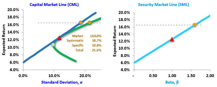
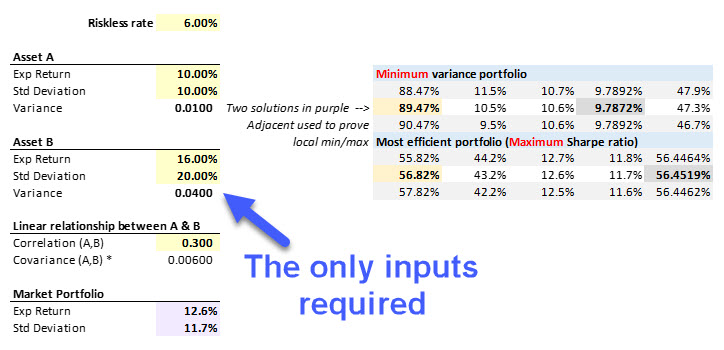
But an illustration might be better, so I quickly added a sheet to our CAPM learning spreadsheet (draft version here, see image below). My spreadsheet is dynamic: you only need to input two assets, their correlation and the riskfree rate. The charts adjust, including I solve for the Market Portfolio (five years ago, I found the analytical solution using mathematica). The plots below happen to assume: For Asset A, μ(A) = +10.0%, σ(A) = 10%. For Asset B, μ(B) =+16.0%, σ(B) = 20.0%. Their correlation, ρ(A,B) = 0.30, and the riskfree rate is 6.0 (primarily to give the plots strong features). The Market Portfolio plots as the red triangle; the Market Portfolio has the highest Sharpe ratio.

The new feature that I added is: you can select the allocation to the Market Portfolio, so that determines your location on the CML. The plot below (left panel) assumes a high-leverage 160.0% allocation the Market Portfolio; it is the orange dot that lies on the CML. There is also plotted a corresponding portfolio on the green PPC: it has the same expected return. Inside the PPC are displayed the risk metrics for this portfolio. In this case, sqrt(18.7%^2 + 10.8%^2) = 21.6% total risk. On the right panel, we see that both of the portfolios on the left locate in the exact same (single) spot on the SML. They both have the same beta of 1.60 per the 160% allocation. And here is the point of the illustration: only portfolios on the CML are "perfectly" well-diversified such that they contain zero specific risk. The portfolio on the PPC offers the same expected return (in this case, +16.5% on both Y axes) and it has the same beta, but it has additional specific risk. In this way, there is a sense in which we can say the portfolios on the green PPC are more diversified as they "get nearer" to the Market Portfolio (which is truly well-diversified and optimal because it has the highest Sharpe ratio, which also means it has zero specific risk). Getting back to the original question, the straight-line CML is also a map to SML/systemic risk but the less efficient portfolios are not.

And this brings me back to my favorite summary distinction of the difference between the CML and SML (and now we can see how the other provider's question contains a glaring mistake): the CML plots only (the most) efficient portfolios, but the SML plots all portfolios (including inefficient portfolios). I hope that's interesting!

2021-05-24-cml-versus-sml-v2.jpg


2021-05-21-model-exhibit.jpg
 
Last edited:

David Harper CFA FRM

David Harper CFA FRM
Subscriber
Note: Durations in CFA and FRM compared

I'd like to clarify duration terminology as it pertains to differences between the CFA and FRM. This forum has hundreds of threads over 12+ years on duration concepts (it's hard to say which links are the best at this point, but I'll maybe come back and curate some best links). Our YouTube channel has a FRM P2.T4 that includes videos on DV01, hedging the DV01, effective duration, modified versus Macaulay duration, and an illustration of all three durations. There are many nuances and further explorations, but here my goal is only to clarify the top-level definitions.

I'll use the simple example of a $100.00 face 20-year zero-coupon bond that currently yields (yield to maturity of) 6.0% per annum. If the yield is 6.0% per annum with continuous compounding, the price is $100.00*exp(-0.060*20) = $30.12. If the yield is 6.0% per annum with annual compounding, the price is $100.00/(1+0.060)^20 = $31.18. Unless otherwise specified, I will assume a continuous compound frequency. Special note: we so often price a bond given the yield (where CPT PV is the final calculator step) that it is easy to forget yield is not actually an input. Yield is the internal rate of return (IRR) assuming the current price. Yield does not determine price; price determines yield. Technical (non-fundamental) factors cause price to fluctuate, therefore yield fluctuates.
  • ∂P/∂y (or Δp/Δy) is the slope of the tangent line at the selected yield. At 6.0% yield, the slope is -$602.39. How do I know that? Because dollar duration is the negated slope, so in this case dollar duration (DD) = P*D = $30.12 price * 20 years = $602.39. Importantly, the "y" in ∂P/∂y is yield and yield is just one of several interest rate factors.
  • Dollar duration (DD; aka, money duration in the CFA) is analytically the product of price and modified duration. Dollar duration (DD) = P*D = $30.12 * 20 = $602.39. Why is it so large? Because it's the (negated) tangent line's slope, so it has the typical first derivative interpretation: DD is the dollar change implied by one unit change in the yield, -∂P/∂y. One unit is 1.0 = 100.0% = 100 * 100 basis points (bps) per 1.0% = 10,000 basis points. So, DD is the dollar change implied by a 100.0% change in yield if we use the straight tangent line which would be a silly thing to do! Recall the constant references to limitations of duration as linear approximation. The linear approximation induces bias at only 5 or 10 or 20 basis points, so 10,000 basis points is literally "off the charts" and not directly meaningful. What is meaningful? The PVBP (aka, DV01) comes to our rescue with a meaningful re-scaling of the DD ...
  • Price value of basis point (aka, dollar value of '01, DV01) is the dollar duration ÷ 10,000. It's the tangent line's slope re-scaled from Δy=100.0% to Δy= 0.010% (one basis point). PVBP = P*D/10,000; in this example, PVBP = $30.12 * 20 / 10,000 = $0.06024. It is the dollar change implied by a one basis point decline in the yield. It is still a linear approximation, but much better because we zoomed in to a small change. In this way, the difference between the highly useful PVBP and the dollar duration is merely scale.
  • Macaulay duration is the bond's weighted average maturity where the weights are each of the bond's cash flow's present value as a percentage of the bond's price. Macaulay duration is tedious however it is reliable and it is analytical. When we can compute the Macaulay duration, it is accurate; we don't approximate by re-pricing the bond. A zero-coupon bond has a Macaulay duration equal to its maturity because it only has one cash flow (hence the popularity of the zero-coupon bond in exam questions, never mind the zero-coupon bond is a reliable primitive). Our 20-year zero-coupon bond has a Macaulay duration of 20.0 years.
  • Modified duration is the measure of interest rate risk. Modified duration is the approximate percentage change in bond price implied by a 1.0% (100 basis point) change in the yield. Just as ∂P/∂y refers to the tangent line's slope which is "infected with price," we divide by price to express the modified duration, D(mod) = -1/P*∂P/∂y. The key relationship between analytical modified and Macaulay duration is the following: modified duration = Macaulay duration / (1 + y/k) where k is the number of compound periods in the year; e.g., k = 1 for annual compounding, k = 2 for semiannual compounding and k = ∞ for continuous compounding. Importantly, if the the compound frequency is continuous then a bond's modified duration equals its Macaulay duration. Notice that T / (1 + y/∞) = T / (1 + 0) = T.
    • If the 6.0% yield is annual compounded, our 20-year bond's Macaulay duration is given by 20.0 / (1 + 6.0%) = 18.868 years.
    • If the 6.0% yield is continuously compounded, our 20-year bond's modified duration is 20.0 years.
  • Effective duration is an approximation of modified duration. Recall the modified duration is a linear approximation, but that's because it is a function of the first derivative; otherwise, modified duration is an exact (analytical or functional) measure of the price sensitivity with respect to the interest rate factor that happens to most often be the yield. We can retrieve it easily whenever we can compute the Macaulay duration, which is the case for any vanilla bond. Otherwise (e.g., bond has an embedded option) we approximate the modified duration by calculating its effective duration. The effective duration approximates the modified duration which itself is a linear approximation. The effective duration is given by [P(-Δy) - P(+Δy)] / (2*Δy) * 1/P. I wrote it this way so you can see that it is essentially similar to ∂P/∂y*1/P where ∂P/∂y ≅ [P(-Δy) - P(+Δy)] / (2*Δy). I've observed that many candidates do not realize that the formula for effective duration is simply slope*1/P. Geometrically, it is the slope of the secant line that is near to the tangent line! Secant's slope approximates the tangent's slope. If you grok the calculus here, I think you'll agree that this is all just one thing! Now we can see how it's not so different. But as you can visualize, there are an almost infinite variety of secants next to the tangent. We arbitrarily choose a nearby secant, but we'd prefer a small delta if the bond is vanilla (i.e., if the bond's cash flows are invariant to rate changes). Although we do not need the effective duration for our example bond, we can compute it:
    • If our arbitrary yield shock is10 basis points such that Δy= 0.10%, then P(-Δy)= $100.00*exp(-5.90%*20)= $30.728, and P(+Δy)= $100.00*exp(-6.10%*20)= $29.523. Effective duration= ($30.728 - $29.523)/0.0020 *1/$30.12= 20.0013 years. Fine approximation!
  • On the terminology (CFA versus FRM)
    • Interest rate factor: The FRM (informed by Tuckman) starts with a general interest rate factor. This is typically the spot rate, forward rate, par rate, or yield. Importantly, the spot, forward and par rates are term structures, or vectors; the par yield curve is a vector of par rates at various maturities, often at six-month or one-month intervals. Only the yield is a single (aka, scalar) value.
    • My above definition of the effective duration is according to the FRM (and to me). The CFA sub-divides this effective duration into either approximate modified duration (if the interest rate factor is the yield) versus effective duration (if the non-vanilla nature of the bond requires a non-yield interest rate factor; i.e., a benchmark yield curve). Personally, I am not keen on this semantic approach because (i) both of these CFA formulas are approximating the modified duration and (ii) I prefer to reserve "effective" for its traditional connotation (e.g., effective convexity is analogous to effective duration), and (iii) we wouldn't anyhow use an inappropriate factor (yield) for certain non-vanilla situations, so we don't really need label-switches to guide us thusly! (the CFA's formula for its approximate modified duration is essentially the same as its effective duration formula). To me, the CFA's approach muddies the terms "approximate" and "effective" where the math gives us natural distinctions. Follow the math, I'd say!
 
Last edited:
Top