BT Notes on Backtesting VaR

[RiskNoob]

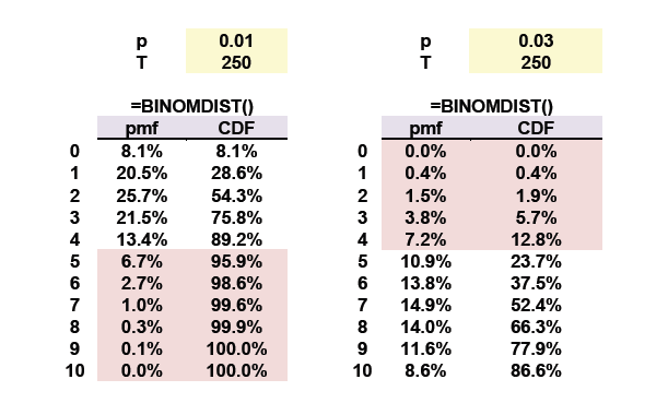
Hi David,

Could you help me out to clarify the basic backtesting? From the last sentence in page 61 in BT notes (Jorion Ch6, Backtesting VaR), it says:

“…In the case of an incorrect model (below right; 3%), the probability of a Type II error is 12.8%”

If the t-statistics from given sample exceed the critical-value (falls into the red-region, 12.8%) in the binomial distribution, the null hypothesis is rejected. and I think this is a ‘good’ decision since the model (null hypothesis) is indeed not correct.

So in my opinion the above sentence could be re-phrased something like:

“…In the case of an incorrect model (below right; 3%), the probability of a NOT making Type II error is at least 12.8%” (it is because Type II error is hard to derive – e.g. failed to reject when the statistics does not exceed the critical value)

Furthermore, the hypothesis test is two-sided, but it is a bit unclear whether it is a two-tailed from the histogram in the notes (same thing can be observed in Jorion’s histogram 6.2) – but it might be due to the binomial distribution which is not continuous.

RiskNoob

 

[RiskNoob]

Please ignore this post, I don't think I specified the null hypothesis correctly from the above post.

The null hypothesis from the Jorion's example is 'given 99% VaR model is correctly calibrated' However, I stated the null hypothesis to be 'the mean of given binomial model is n*p (which is the classical t-test for mean, and n is the number of days)...

Ouch
RiskNoob

 

[RiskNoob]

Please ignore this post, I don't think I specified the null hypothesis correctly from the above post.

The null hypothesis from the Jorion's example is 'given 99% VaR model is correctly calibrated' However, I stated the null hypothesis to be 'the mean of given binomial model is n*p (which is the classical t-test for mean, and n is the number of days)...

Ouch
RiskNoob

The above posts from myself are quite confusing - I think I got too relaxed in the holiday period and totally confused myself. To summarize the backtesting concept above,

Null hypothesis: Given 99% (alpha=0.01) VaR model is correctly calibrated

Test case 1: when the number exceedences are calculated based on the model which is indeed correct(p=0.01), the probability of exceeding the critical value (from the two-tailed 95% null hypothesis test of binomial mean with alpha=0.01), or probability of rejecting the true model (type 1 error) is approx. 10.8%

Test case 2: when the number exceedences are calculated based on the model which is indeed incorrect(say p=0.03), the probability of NOT exceeding the critical value (from the two-tailed 95% null hypothesis test of binomial mean with alpha=0.01, notice alpha != p in this case), or probability of accepting the false model (type 2 error) is approx. 12.8%

RiskNoob

 

[Arsalan Amin]

Hi, I am not sure if I should be posting on such an old thread but could not find another thread relating to the notes on this chapter.

I had a question regarding the LOS: Describe the process of model verification based on exceptions or failure rates.

In Jorion's backtesting example relating to Type 1 and Type 2 errors, I can't understand why are we looking at the exceptions above 4 rather than 2.5 (or 3 to round off) since a 99% VAR would be expected to be exceeded 1% of the times which would be (250*0.01) 2.5 and not 4.

I'm not that technically sound on this topic so could be a simple concept which I have failed to understand

 

[Arsalan Amin]

Hi @David Harper CFA FRM, dont expect a lot of people to see the above post since its an old thread.

Was hoping if you could have a look at it. Thanks. I just cant seem to understand why did we look at the number of exceptions above 4 for P= 0.01 and 0.03 rather than 2.5 or 3.

 

[David Harper CFA FRM]

Its a great question, I did not understand it either when I first read it. Statistically speaking, Jorion makes two arbitrary choices: the cutoff of four (4) exceptions and the assumption that a "bad" 99.0% VaR model would exhibit an exception rate of 3.0%. There is nothing magic about the four, except that it happens to coincide with Basel's choice for the cutoff, which is a good enough reason, as the Committee clearly gave it careful consideration (Here is the BCBS document with the detailed statistics: http://trtl.bz/bcbs22-pdf).

It's a two-step illustration in Jorion. First, he assume a "good" 99% VaR model which, if perfect, would exhibit 1%*250 = 2.5 exceptions per year. His point here is that we can't overcome a trade-off. Given a good model, there is only the possibility of a Type I error and the probabilities of such an error at various cutoffs are (eg)

• At 3 cutoffs (i.e., Green Zone is 3 exceptions or less): 1 - BINOM.DIST(3, 250, 0.01, true) = 24.19%
• At 4 cutoffs (i.e., Green Zone is 4 exceptions or less): 1 - BINOM.DIST(4, 250, 0.01, true) = 10.78%; i.e., as the cutoff is four or less, inclusive, this error probability refers to five or greater, inclusive
• At 5 cutoffs (i.e., Green Zone is 5 exceptions or less): 1 - BINOM.DIST(5, 250, 0.01, true) = 4.12%

Given a mean of 2.5, there is nothing magically superior to 4; it's just a trade-off judgment. With respect to this perfect (good) model, if we error there is only the possibility of a Type I. We can raise the cutoff and reduce the probability of a Type I ... HOWEVER, we aren't done. We need to consider the other mistake. The problem here is that, while there is only one perfect model, there are many possible bad models. A nearly good 99% VaR model would exhibit 2% exceptions; a terrible 99% model would exhibit 90% exhibits, or less (worse). Jorion simply arbitrarily decides to illustrate a bad 99% VaR model by assuming its exception rate is 97% (not terrible, but not really great either). Then the point is to illustrate the probability of a Type II error conditional on this one, arbitrary bad model. But we already selected the cutoff. So now the Prob of a Type II error, given our selected cutoff and conditional on this particular bad model, is given by BINOM.DIST(4, 250, 0.03, true) =12.82%. However, we can imagine other VaR models given this same cutoff:

• Given cutoff of 4 inclusive, bad model actually 98%: BINOM.DIST(4, 250, 0.02, true) = 43.87%
• Given cutoff of 4 inclusive, bad model actually 97%: BINOM.DIST(4, 250, 0.03, true) = 12.82%
• Given cutoff of 4 inclusive, bad model actually 96%: BINOM.DIST(4, 250, 0.04, true) = 2.70%

It's all to illustrate the trade-off. But the cutoff obviously needs to be the same for both because we won't know a priori if the model is good or bad, it's not like we can have a higher cutoff for good models and a lower cutoff for bad models. We might be tempted to increase the cutoff to 5, which lowers the Prob of a Type I error to 4.12% (yay!), but then if the bad model is 97% (which ain't too bad really!) we increase the Prob of Type II error to fully 23.73%. I hope that explains!

 

[Arsalan Amin]

Thanks @David Harper CFA FRM. It all makes sense to me now.

 

[Rohit]

@David Harper CFA FRM for Jorian's back testing VAR example - what does the pink shaded region signify ?

Example - if 99% VAR over 1 year horizon (250 days) is 10 mill, expected exceptions is 2.5 days/ per year (0.05*250=2.5 or 3 approx.). So we expect to lose >10 mill on 3 trading days of the year.
Let's say over 250 days we flag each day on whether it exceeded 10 mill or not.

If we see <= 3 exceptions in a year then we are within the expectation (3 days) and accept null hypothesis (i.e. accept model) else we reject the model.

I do not understand why in the notes the pink shaded region shows 5 or more exceptions highlighted.

Please help.

 

[David Harper CFA FRM]

Hi @Rohit please see my answer last week, in case this helps https://forum.bionicturtle.com/threads/l2-t5-57-value-at-risk-var-backtest.3602/#post-47586

It's my fault as these are not sufficiently explained, sorry. (My example parrots Jorion). Your scenario is correct. If we have a 99.0% VaR model, the null hypothesis is "model is good (accurate)." The left-hand panel illustrates a binomial distribution based on this good model (i.e., p = 0.01) over 250 trading days. The red/pink region simply means to illustrate the implications of a cutoff selected at 4 exceptions (following Basel II but only as the yellow zone; the red zone cutoff is 9); i.e., 5 or more exceptions and we consider rejecting the null. If we decided to reject the null at 5 exceptions, that's a probability of a Type I error of 10.8% (which is a low confidence/high significance level setting). On the right panel is the other error that can be made given the same cutoff: if we accept at 4 exceedences (on the cutoff), we have a surprisingly high chance of accepting a bad model (Type II error). So the pink regions are meant to illustrate the two errors, and their necessary trade-off, that can be made given the same cutoff at four. (the problem with the illustration is selecting the bad model on the right: we could chose a different p = X scenario). I hope that clarifies, we need to improve this in the notes obviously ...

 

[Rohit]

@David Harper CFA FRM

As per above I am trying to understand via hypothesis test - 99%, 2 tail test. Please tell me if my understanding is correct?

H0 = 0.01*250 = 2.5 exceptions expected

Ha = 5 exceptions (let's assume this is the alt hypothesis)

99% 2 tail hypothesis test t-critical = 2.54 (reject null if >2.54 or <-2.54)

test statistic t-stat = 5-2.5/sqrt(250*0.01*0.99) = 1.589 ........for binomial dist, large sample size std error is std dev

t-stat does not breach the t-critical hence we accept null at 5 exceptions.
If we rejected this, then it would lead to Type 1 error

On the other hand at Ha = 7 exceptions we breach t-critical, if we would have accepted null then this would be Type II error

Thanks !

 

[David Harper CFA FRM]

Hi @Rohit Yes I mostly agree! (just two comments):

• Agree, the null is: H0 = 0.01*250 = 2.5 exceptions expected. And just a reminder, this is where we are assuming the 99.0% VaR model is good; put another way, this is where we are assuming p = 0.010.
  
• Ha = 5 is not exactly the alternative (sorry). On a technical point, the Null contains the equal sign ("=") so the alternative never does. The alternative is everything else, so if the null is µ=2.5, then the two-tailed null is given by H(a): µ<>2.5
• For the 99.0% 2-tailed critical t-value I get =T.INV.2T(1%,249) = 2.59571776, assuming 250 sample so there are 249 = n - 1 degrees of freedom. What does this mean? This means that in a student's t distribution with 249 df, at +2.59 standard deviations (the quantile), outside that area is only the 0.5% tail on the right (and the other 0.5% tail to the left of - 2.59571776 standard deviations).
• Re: test statistic t-stat = 5-2.5/sqrt(250*0.01*0.99) = 1.589. Yes, exactly (if we assume that we observe 5 exceptions, of course)! (5 - 2.5) is the distance from our observation to the expected mean, and this is divided by the standard deviation of the binomal in order to create a standardized standard deviation. In short, this observation is only 1.589 standard deviations away from the expected mean (not where we expect, but very possible on a given random trial).
• Agree, because 1.589 < 2.595, we fail to reject. However, we risk a type II error (mistakenly accepting a bad model). Having failed to reject, we can only commit a Type II error. But please note, the 99.0% VaR is coincident to our choice of a 2-tailed 99.0% significance test. We could decide to test this 99.0% VaR instead at 95%: critical t = =T.INV.2T(5%,249) = 1.970 and because 1.589 < 1.970 we fail to reject even at the lower confidence.
• If however we observe 7 exceptions, then test statistic = 2.80 and we do reject at 99.0% 2-tailed confidence. Because we rejected the null, our possible error is Type I. I hope that clarifies!