BT Notes on Backtesting VaR

RiskNoob

Active Member
Hi David,

Could you help me out to clarify the basic backtesting? From the last sentence in page 61 in BT notes (Jorion Ch6, Backtesting VaR), it says:

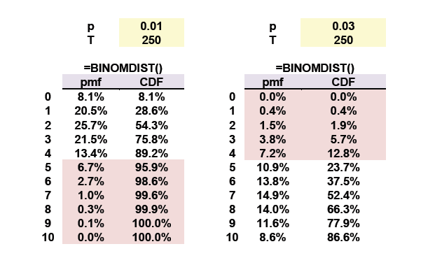
“…In the case of an incorrect model (below right; 3%), the probability of a Type II error is 12.8%”

If the t-statistics from given sample exceed the critical-value (falls into the red-region, 12.8%) in the binomial distribution, the null hypothesis is rejected. and I think this is a ‘good’ decision since the model (null hypothesis) is indeed not correct.

So in my opinion the above sentence could be re-phrased something like:

“…In the case of an incorrect model (below right; 3%), the probability of a NOT making Type II error is at least 12.8%” (it is because Type II error is hard to derive – e.g. failed to reject when the statistics does not exceed the critical value)

Furthermore, the hypothesis test is two-sided, but it is a bit unclear whether it is a two-tailed from the histogram in the notes (same thing can be observed in Jorion’s histogram 6.2) – but it might be due to the binomial distribution which is not continuous.

RiskNoob
 

RiskNoob

Active Member
Please ignore this post, I don't think I specified the null hypothesis correctly from the above post.

The null hypothesis from the Jorion's example is 'given 99% VaR model is correctly calibrated' However, I stated the null hypothesis to be 'the mean of given binomial model is n*p (which is the classical t-test for mean, and n is the number of days)...

Ouch :confused:
RiskNoob
 

RiskNoob

Active Member
Please ignore this post, I don't think I specified the null hypothesis correctly from the above post.

The null hypothesis from the Jorion's example is 'given 99% VaR model is correctly calibrated' However, I stated the null hypothesis to be 'the mean of given binomial model is n*p (which is the classical t-test for mean, and n is the number of days)...

Ouch :confused:
RiskNoob


The above posts from myself are quite confusing - I think I got too relaxed in the holiday period and totally confused myself. To summarize the backtesting concept above,

Null hypothesis: Given 99% (alpha=0.01) VaR model is correctly calibrated

Test case 1: when the number exceedences are calculated based on the model which is indeed correct(p=0.01), the probability of exceeding the critical value (from the two-tailed 95% null hypothesis test of binomial mean with alpha=0.01), or probability of rejecting the true model (type 1 error) is approx. 10.8%

Test case 2: when the number exceedences are calculated based on the model which is indeed incorrect(say p=0.03), the probability of NOT exceeding the critical value (from the two-tailed 95% null hypothesis test of binomial mean with alpha=0.01, notice alpha != p in this case), or probability of accepting the false model (type 2 error) is approx. 12.8%

RiskNoob
 

Arsalan Amin

New Member
Hi, I am not sure if I should be posting on such an old thread but could not find another thread relating to the notes on this chapter.

I had a question regarding the LOS: Describe the process of model verification based on exceptions or failure rates.

In Jorion's backtesting example relating to Type 1 and Type 2 errors, I can't understand why are we looking at the exceptions above 4 rather than 2.5 (or 3 to round off) since a 99% VAR would be expected to be exceeded 1% of the times which would be (250*0.01) 2.5 and not 4.

I'm not that technically sound on this topic so could be a simple concept which I have failed to understand :D
 
Last edited:

Arsalan Amin

New Member
Hi @David Harper CFA FRM, dont expect a lot of people to see the above post since its an old thread.

Was hoping if you could have a look at it. Thanks. I just cant seem to understand why did we look at the number of exceptions above 4 for P= 0.01 and 0.03 rather than 2.5 or 3.
 

David Harper CFA FRM

David Harper CFA FRM
Subscriber
Its a great question, I did not understand it either when I first read it. Statistically speaking, Jorion makes two arbitrary choices: the cutoff of four (4) exceptions and the assumption that a "bad" 99.0% VaR model would exhibit an exception rate of 3.0%. There is nothing magic about the four, except that it happens to coincide with Basel's choice for the cutoff, which is a good enough reason, as the Committee clearly gave it careful consideration (Here is the BCBS document with the detailed statistics: http://trtl.bz/bcbs22-pdf).

It's a two-step illustration in Jorion. First, he assume a "good" 99% VaR model which, if perfect, would exhibit 1%*250 = 2.5 exceptions per year. His point here is that we can't overcome a trade-off. Given a good model, there is only the possibility of a Type I error and the probabilities of such an error at various cutoffs are (eg)
  • At 3 cutoffs (i.e., Green Zone is 3 exceptions or less): 1 - BINOM.DIST(3, 250, 0.01, true) = 24.19%
  • At 4 cutoffs (i.e., Green Zone is 4 exceptions or less): 1 - BINOM.DIST(4, 250, 0.01, true) = 10.78%; i.e., as the cutoff is four or less, inclusive, this error probability refers to five or greater, inclusive
  • At 5 cutoffs (i.e., Green Zone is 5 exceptions or less): 1 - BINOM.DIST(5, 250, 0.01, true) = 4.12%
Given a mean of 2.5, there is nothing magically superior to 4; it's just a trade-off judgment. With respect to this perfect (good) model, if we error there is only the possibility of a Type I. We can raise the cutoff and reduce the probability of a Type I ... HOWEVER, we aren't done. We need to consider the other mistake. The problem here is that, while there is only one perfect model, there are many possible bad models. A nearly good 99% VaR model would exhibit 2% exceptions; a terrible 99% model would exhibit 90% exhibits, or less (worse). Jorion simply arbitrarily decides to illustrate a bad 99% VaR model by assuming its exception rate is 97% (not terrible, but not really great either). Then the point is to illustrate the probability of a Type II error conditional on this one, arbitrary bad model. But we already selected the cutoff. So now the Prob of a Type II error, given our selected cutoff and conditional on this particular bad model, is given by BINOM.DIST(4, 250, 0.03, true) =12.82%. However, we can imagine other VaR models given this same cutoff:
  • Given cutoff of 4 inclusive, bad model actually 98%: BINOM.DIST(4, 250, 0.02, true) = 43.87%
  • Given cutoff of 4 inclusive, bad model actually 97%: BINOM.DIST(4, 250, 0.03, true) = 12.82%
  • Given cutoff of 4 inclusive, bad model actually 96%: BINOM.DIST(4, 250, 0.04, true) = 2.70%
It's all to illustrate the trade-off. But the cutoff obviously needs to be the same for both because we won't know a priori if the model is good or bad, it's not like we can have a higher cutoff for good models and a lower cutoff for bad models:rolleyes:. We might be tempted to increase the cutoff to 5, which lowers the Prob of a Type I error to 4.12% (yay!), but then if the bad model is 97% (which ain't too bad really!) we increase the Prob of Type II error to fully 23.73%. I hope that explains!
 
Last edited:

Rohit

Member
@David Harper CFA FRM for Jorian's back testing VAR example - what does the pink shaded region signify ?

Example - if 99% VAR over 1 year horizon (250 days) is 10 mill, expected exceptions is 2.5 days/ per year (0.05*250=2.5 or 3 approx.). So we expect to lose >10 mill on 3 trading days of the year.
Let's say over 250 days we flag each day on whether it exceeded 10 mill or not.

If we see <= 3 exceptions in a year then we are within the expectation (3 days) and accept null hypothesis (i.e. accept model) else we reject the model.

I do not understand why in the notes the pink shaded region shows 5 or more exceptions highlighted.

Please help.
 

David Harper CFA FRM

David Harper CFA FRM
Subscriber
Hi @Rohit please see my answer last week, in case this helps https://forum.bionicturtle.com/threads/l2-t5-57-value-at-risk-var-backtest.3602/#post-47586

It's my fault as these are not sufficiently explained, sorry. (My example parrots Jorion). Your scenario is correct. If we have a 99.0% VaR model, the null hypothesis is "model is good (accurate)." The left-hand panel illustrates a binomial distribution based on this good model (i.e., p = 0.01) over 250 trading days. The red/pink region simply means to illustrate the implications of a cutoff selected at 4 exceptions (following Basel II but only as the yellow zone; the red zone cutoff is 9); i.e., 5 or more exceptions and we consider rejecting the null. If we decided to reject the null at 5 exceptions, that's a probability of a Type I error of 10.8% (which is a low confidence/high significance level setting). On the right panel is the other error that can be made given the same cutoff: if we accept at 4 exceedences (on the cutoff), we have a surprisingly high chance of accepting a bad model (Type II error). So the pink regions are meant to illustrate the two errors, and their necessary trade-off, that can be made given the same cutoff at four. (the problem with the illustration is selecting the bad model on the right: we could chose a different p = X scenario). I hope that clarifies, we need to improve this in the notes obviously ...
0118-backtest-type-error.png
 

Rohit

Member
@David Harper CFA FRM

As per above I am trying to understand via hypothesis test - 99%, 2 tail test. Please tell me if my understanding is correct?

H0 = 0.01*250 = 2.5 exceptions expected

Ha = 5 exceptions (let's assume this is the alt hypothesis)

99% 2 tail hypothesis test t-critical = 2.54 (reject null if >2.54 or <-2.54)

test statistic t-stat = 5-2.5/sqrt(250*0.01*0.99) = 1.589 ........for binomial dist, large sample size std error is std dev

t-stat does not breach the t-critical hence we accept null at 5 exceptions.
If we rejected this, then it would lead to Type 1 error

On the other hand at Ha = 7 exceptions we breach t-critical, if we would have accepted null then this would be Type II error

Thanks !
 
Last edited:

David Harper CFA FRM

David Harper CFA FRM
Subscriber
Hi @Rohit Yes I mostly agree! (just two comments):
  • Agree, the null is: H0 = 0.01*250 = 2.5 exceptions expected. And just a reminder, this is where we are assuming the 99.0% VaR model is good; put another way, this is where we are assuming p = 0.010.
  • Ha = 5 is not exactly the alternative (sorry). On a technical point, the Null contains the equal sign ("=") so the alternative never does. The alternative is everything else, so if the null is µ=2.5, then the two-tailed null is given by H(a): µ<>2.5
  • For the 99.0% 2-tailed critical t-value I get =T.INV.2T(1%,249) = 2.59571776, assuming 250 sample so there are 249 = n - 1 degrees of freedom. What does this mean? This means that in a student's t distribution with 249 df, at +2.59 standard deviations (the quantile), outside that area is only the 0.5% tail on the right (and the other 0.5% tail to the left of - 2.59571776 standard deviations).
  • Re: test statistic t-stat = 5-2.5/sqrt(250*0.01*0.99) = 1.589. Yes, exactly (if we assume that we observe 5 exceptions, of course)! (5 - 2.5) is the distance from our observation to the expected mean, and this is divided by the standard deviation of the binomal in order to create a standardized standard deviation. In short, this observation is only 1.589 standard deviations away from the expected mean (not where we expect, but very possible on a given random trial).
  • Agree, because 1.589 < 2.595, we fail to reject. However, we risk a type II error (mistakenly accepting a bad model). Having failed to reject, we can only commit a Type II error. But please note, the 99.0% VaR is coincident to our choice of a 2-tailed 99.0% significance test. We could decide to test this 99.0% VaR instead at 95%: critical t = =T.INV.2T(5%,249) = 1.970 and because 1.589 < 1.970 we fail to reject even at the lower confidence.
  • If however we observe 7 exceptions, then test statistic = 2.80 and we do reject at 99.0% 2-tailed confidence. Because we rejected the null, our possible error is Type I. I hope that clarifies!


Top